Tutorial: OpenCv (Python) Basics

Tutorial: OpenCV (Python) Basics

Preparation

Basics of Python & Numpy

Skip this if you already know about Python programming

Python Basics

Python_Numpy | DLIPykkim.gitbook.io

Numpy Basics

Python_Numpy | DLIPykkim.gitbook.io

Configuration

Prepare the environment as

1. Visual Studio Code

2. Python Environment (>3.7)

3. OpenCV Installation

Follow the tutorial for installation

Tutorial: Installation for Py OpenCV | DLIPykkim.gitbook.io

Source code and images

Download

Download the tutorial source code and image files.

• Tutorial Code in *.ipynb

• Test Image Files

Project and Data Folder

The downloaded images should be saved in

• Image Folder: C:\Users\yourID\source\repos\DLIP\Image\

The python opencv tutorial is operated under the project folder

• Python File Folder: C:\Users\yourID\source\repos\DLIP\Tutorial\PyOpenCV\

The visual studio code open project at DLIP folder

• Project Folder: C:\Users\yourID\source\repos\DLIP\

Running the source code

This tutorial code is based on Google Colab Notebook.

When running the code, you can select from two options

1. (Recommended) Download the notebook file (*.ipynb) and run in VS.Code

2. Run directly on Google Colab

---

Basic Image Processing

(*.py) Read / Write / Display Image and Video

You must Read Documentation!! link

1. Download HGU logo image and rename HGU_logo.jpg

   • Image Link: HGU_logo

   • Image Folder: C:\Users\yourID\source\repos\DLIP\Image\

2. Create a new python source file in Visual Studio Code

   • File Name: DLIP_Tutorial_OpenCV_Image.py and DLIP_Tutorial_OpenCV_Video.py

   • Project Folder: C:\Users\yourID\source\repos\DLIP\Tutorial\PyOpenCV

3. Compile and run.

DLIP_Tutorial_OpenCV_Image.py

import cv2 as cv

# Read image
HGU_logo = 'Image/HGU_logo.jpg'
src = cv.imread(HGU_logo)
src_gray = cv.imread(HGU_logo, cv.IMREAD_GRAYSCALE)

# Write image
HGU_logo_name = 'writeImage.jpg'
cv.imwrite(HGU_logo_name, src)

# Display image
cv.namedWindow('src', cv.WINDOW_AUTOSIZE)
cv.imshow('src', src)

cv.namedWindow('src_gray', cv.WINDOW_AUTOSIZE)
cv.imshow('src_gray', src_gray)

cv.waitKey(0)

DLIP_Tutorial_OpenCV_Video.py

---

(*.ipyn) Read / Write / Display Image and Video

Import OpenCV Library

import numpy as np
import cv2 as cv
from matplotlib import pyplot as plt

---

(for COLAB only) Upload Image Files in Colab server

Skip this if you are using Visual Studio Code

Read how to load image file in Colab

Google Codelab | DLIPykkim.gitbook.io

Other Option: Upload image file to Colab server from local drive

from google.colab import files
uploaded=files.upload()

Read Image File

# Load image
img = cv.imread('Image/HGU_logo.jpg')

Display Image using matplot plt.imshow()

This tutorial will use matplotlib functions for *.ipyn files. This method is recommended for showing images. This works for both *.py and *.ipyn files.

matplotlib has different rgb order than OpenCV

• matplot: R-G-B

• OpenCV: G-B-R

# Load image
img = cv.imread('Image/HGU_logo.jpg')


# Show Image using matplotlib
# matplotlib에서 rgb 채널 순서가 다름
# matplot:  R-G-B
# OpenCV:   B-G-R
imgPlt = cv.cvtColor(img, cv.COLOR_BGR2RGB)

plt.imshow(imgPlt),plt.title('Original')
plt.xticks([]), plt.yticks([])
plt.show()

Display Image: (for .py only) OpenCV imshow()

This is only for *.py file. Python files running on local drive supports OpenCV cv.imshow()

Notebook files such as Colab and Jupyter does NOT support OpenCV cv.imshow()

This does not work on *.ipyn file

# Load image
img = cv.imread('Image/HGU_logo.jpg')

# Show Image using colab imshow
cv.imshow('source',img)
cv.waitKey(0)

Display Image: (for Colab only) cv2_imshow()

CoLAB provides a similar function called cv2_imshow(). But this is NOT recommended method.

Import

from google.colab.patches import cv2_imshow as cv_imshow

# Import COLAB imshow() 
from google.colab.patches import cv2_imshow as cv_imshow

# Load image
img = cv.imread('Image/HGU_logo.jpg')

# Show Image using colab imshow
cv_imshow(img) 

Capturing Video

Using webcam in notebook(colab, jupyter) requires more complex setup.

cv.VideoCapture(0) is NOT available in Colab.

Spatial Filter

• Box filter

• Gaussian filter

• Median filter

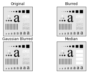
cv.blur(src, ksize[, dst[, anchor[, borderType]]])
cv.GaussianBlur(src, ksize, sigmaX[, dst[, sigmaY[, borderType]]])
cv.medianBlur(src, ksize[, dst])

Example Code

# Load image
img = cv.imread('Image/Pattern_original.tif')

# Spatial Filter
blur = cv.blur(img,(5,5))
gblur = cv.GaussianBlur(img,(5,5),0)
median = cv.medianBlur(img,5)

# Plot results
plt.subplot(221),plt.imshow(img),plt.title('Original')
plt.xticks([]), plt.yticks([])
plt.subplot(222),plt.imshow(blur),plt.title('Blurred')
plt.xticks([]), plt.yticks([])
plt.subplot(223),plt.imshow(gblur),plt.title('Gaussian Blurred')
plt.xticks([]), plt.yticks([])
plt.subplot(224),plt.imshow(median),plt.title('Median')
plt.xticks([]), plt.yticks([])
plt.show()

image

---

Thresholding

• Thresholding

cv.threshold(src, thresh, maxval, type[, dst])

Manual Local Threshold

Example Code

# Open Image
img = cv.imread('Image/coins.png',0)

thVal=127

# Apply Thresholding
ret,thresh1 = cv.threshold(img,thVal,255,cv.THRESH_BINARY)
ret,thresh2 = cv.threshold(img,thVal,255,cv.THRESH_BINARY_INV)

# Plot results
titles = ['Original Image','BINARY','BINARY_INV']
images = [img, thresh1, thresh2]

for i in range(3):
    plt.subplot(1,3,i+1),plt.imshow(images[i],'gray',vmin=0,vmax=255)
    plt.title(titles[i])
    plt.xticks([]),plt.yticks([])
plt.show()

image

Adaptive Threshold

• Adaptive Threshold

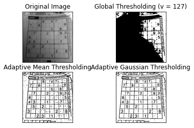
cv.adaptiveThreshold(src, maxValue, adaptiveMethod, thresholdType, blockSize, C[, dst])

Example code

# Read image
img = cv.imread('Image/sudoku.jpg',0)

# Preprocessing
img = cv.medianBlur(img,5)

# Global threshold
ret,th1 = cv.threshold(img,127,255,cv.THRESH_BINARY)

# Local threshold
th2 = cv.adaptiveThreshold(img,255,cv.ADAPTIVE_THRESH_MEAN_C,\
            cv.THRESH_BINARY,11,2)
th3 = cv.adaptiveThreshold(img,255,cv.ADAPTIVE_THRESH_GAUSSIAN_C,\
            cv.THRESH_BINARY,11,2)

# Plot results
titles = ['Original Image', 'Global Thresholding (v = 127)',
            'Adaptive Mean Thresholding', 'Adaptive Gaussian Thresholding']
images = [img, th1, th2, th3]

for i in range(4):
    plt.subplot(2,2,i+1),plt.imshow(images[i],'gray')
    plt.title(titles[i])
    plt.xticks([]),plt.yticks([])
plt.show()

image

Plot Histogram

• calcHist

hist=cv.calcHist(images, channels, mask, histSize, ranges[, hist[, accumulate]])

Example Code

# Open Image
img = cv.imread('Image/coins.png',0)

histSize = 256
histRange = (0, 256) # the upper boundary is exclusive
b_hist = cv.calcHist(img, [0], None, [histSize], histRange, False)

hist_w = 512
hist_h = 400
bin_w = int(round( hist_w/histSize ))
histImage = np.zeros((hist_h, hist_w, 3), dtype=np.uint8)

# Normalize histogram output
cv.normalize(b_hist, b_hist, alpha=0, beta=hist_h, norm_type=cv.NORM_MINMAX)

for i in range(1, histSize):
    cv.line(histImage, ( bin_w*(i-1), hist_h - int(b_hist[i-1]) ),
            ( bin_w*(i), hist_h - int(b_hist[i]) ),
            ( 255, 0, 0), thickness=2)

# Plot Results
#cv.imshow('Source image', img)
#cv.imshow('calcHist Demo', histImage)

plt.subplot(2,2,1),plt.imshow(img, 'gray')
plt.title('Source image')
plt.xticks([]),plt.yticks([])
plt.subplot(2,2,2),plt.imshow(histImage)
plt.title('CalcHist image')
plt.xticks([]),plt.yticks([])
plt.show()

Morphology

• Erode

• Dilate

• morphologyEx

cv.erode(src, kernel[, dst[, anchor[, iterations[, borderType[, borderValue]]]]])
cv.dilate(src, kernel[, dst[, anchor[, iterations[, borderType[, borderValue]]]]])
cv.morphologyEx(src, op, kernel[, dst[, anchor[, iterations[, borderType[, borderValue]]]]])

Example Code

# Open Image
src = cv.imread('Image/coins.png',0)


# Threshold
ret,thresh1 = cv.threshold(src,127,255,cv.THRESH_BINARY)
img=thresh1

# Structure Element for Morphology
cv.getStructuringElement(cv.MORPH_RECT,(5,5))
kernel = np.ones((5,5),np.uint8)

# Morphology
erosion = cv.erode(img,kernel,iterations = 1)
dilation = cv.dilate(img,kernel,iterations = 1)
opening = cv.morphologyEx(img, cv.MORPH_OPEN, kernel)
closing = cv.morphologyEx(img, cv.MORPH_CLOSE, kernel)


# Plot results
titles = ['Original ', 'Opening','Closing']
images = [src, opening, closing]

for i in range(3):
    plt.subplot(1,3,i+1),plt.imshow(images[i],'gray')
    plt.title(titles[i])
    plt.xticks([]),plt.yticks([])
plt.show()

image

---

Color Segmentation (InRange)

• inRange

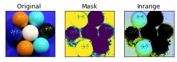
dst= cv2.inRange(src, lowerb, upperb, dst=None)

Example code

# Open Image in RGB
img = cv.imread('Image/color_ball.jpg')

# Convert BRG to HSV 
hsv = cv.cvtColor(img, cv.COLOR_BGR2HSV)

# matplotlib: cvt color for display
imgPlt = cv.cvtColor(img, cv.COLOR_BGR2RGB)

# Color InRange()
lower_range = np.array([100,128,0])
upper_range = np.array([215,255,255])
dst_inrange = cv.inRange(hsv, lower_range, upper_range)

# Mask selected range
mask = cv.inRange(hsv, lower_range, upper_range)
dst = cv.bitwise_and(hsv,hsv, mask= mask)

# Plot Results
titles = ['Original ', 'Mask','Inrange']
images = [imgPlt, mask, dst]

for i in range(3):
    plt.subplot(1,3,i+1),plt.imshow(images[i])
    plt.title(titles[i])
    plt.xticks([]),plt.yticks([])
plt.show()

image

---

Edge & Line & Circle Detection

Edge Detection

• Canny

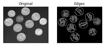
cv.Canny(image, threshold1, threshold2[, edges[, apertureSize[, L2gradient]]])

Example code 1

# Load image
img = cv.imread('Image/coins.png',0)

# Apply Canndy Edge
edges = cv.Canny(img,50,200)

# Plot Results
#cv.imshow('Edges',edges)
titles = ['Original','Edges']
images = [img, edges]
for i in range(2):
    plt.subplot(1,2,i+1),plt.imshow(images[i],'gray')
    plt.title(titles[i])
    plt.xticks([]),plt.yticks([])
plt.show()

Example code 2

# Load image
img = cv.imread('Image/coins.png',0)
# Apply Thresholding then Canndy Edge
thVal=127
ret,thresh1 = cv.threshold(img,thVal,255,cv.THRESH_BINARY)
edges = cv.Canny(thresh1,50,200)

# Plot Results
#cv.imshow('Edges',edges)
titles = ['Original','Edges']
images = [img, edges]
for i in range(2):
    plt.subplot(1,2,i+1),plt.imshow(images[i],'gray')
    plt.title(titles[i])
    plt.xticks([]),plt.yticks([])
plt.show()
    

image

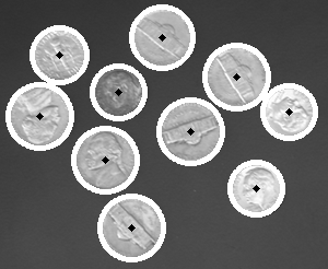
Circle Detection

HoughCircles

cv.HoughCircles(image, method, dp, minDist[, circles[, param1[, param2[, minRadius[, maxRadius]]]]])

Example code

# Read Image
src = cv.imread('Image/coins.png')

# Convert it to grayscale:
gray = cv.cvtColor(src, cv.COLOR_BGR2GRAY)


# Reduce noise and avoid false circle detection
gray = cv.medianBlur(gray, 5)


# Hough Circle Transform
rows = gray.shape[0]
circles = cv.HoughCircles(gray, cv.HOUGH_GRADIENT, 1, rows / 8,
                               param1=100, param2=30,
                               minRadius=1, maxRadius=30)

# Draw circle
if circles is not None:
    circles = np.uint16(np.around(circles))
    for i in circles[0, :]:
        center = (i[0], i[1])
        # Draw circle center
        cv.circle(src, center, 1, (0, 100, 100), 3)
        # Draw circle outline
        radius = i[2]
        cv.circle(src, center, radius, (255, 0, 0), 3)


# Plot images
titles = ['Original with Circle Detected']
srcPlt=cv.cvtColor(src,cv.COLOR_BGR2RGB)
plt.imshow(srcPlt)
plt.title(titles)
plt.xticks([]),plt.yticks([])
plt.show()

image

Line Detection

• HoughLines

cv.HoughLines(image, rho, theta, threshold[, lines[, srn[, stn[, min_theta[, max_theta]]]]])
cv.HoughLinesP(image, rho, theta, threshold[, lines[, minLineLength[, maxLineGap]]])

Example code

# Load image
img = cv.imread('Image/sudoku.jpg',0)  # Gray scale image

# Canny Edge Detection
dst = cv.Canny(img, 50, 200, None, 3)

# Copy edges to the images that will display the results in BGR
cdst = cv.cvtColor(dst, cv.COLOR_GRAY2BGR)
cdstP = np.copy(cdst)

# (Option 1) HoughLines
lines = cv.HoughLines(dst, 1, np.pi / 180, 150, None, 0, 0)
if lines is not None:
    for i in range(0, len(lines)):
        rho = lines[i][0][0]
        theta = lines[i][0][1]
        a = np.cos(theta)
        b = np.sin(theta)
        x0 = a * rho
        y0 = b * rho
        pt1 = (int(x0 + 1000*(-b)), int(y0 + 1000*(a)))
        pt2 = (int(x0 - 1000*(-b)), int(y0 - 1000*(a)))
        cv.line(cdst, pt1, pt2, (0,0,255), 3, cv.LINE_AA)

# (Option 2) HoughLinesP
linesP = cv.HoughLinesP(dst, 1, np.pi / 180, 50, None, 50, 10)
if linesP is not None:
  for i in range(0, len(linesP)):
    l = linesP[i][0]
    cv.line(cdstP, (l[0], l[1]), (l[2], l[3]), (0,0,255), 3, cv.LINE_AA)

# Plot Results
#cv.imshow("Source", img)
#cv.imshow("Detected Lines (in red) - Standard Hough Line Transform", cdst)
#cv.imshow("Detected Lines (in red) - Probabilistic Line Transform", cdstP)
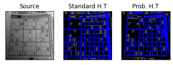
titles = ['Source','Standard H.T','Prob. H.T']
images = [img, cdst, cdstP]
for i in range(3):
    plt.subplot(1,3,i+1),plt.imshow(images[i],'gray')
    plt.title(titles[i])
    plt.xticks([]),plt.yticks([])
plt.show()
    

image

---

Exercise

Beginner Level Exercise

Exercise 1

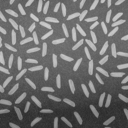
Apply Blur filters, Thresholding and Morphology methods on given images for object segmentation.

download test image

image

Example 2

Choose the appropriate InRange conditions to segment only ' Blue colored ball'. Draw the contour and a box over the target object. Repeat for Red, and Yellow balls

download test image

Example 3

Detect Pupil/Iris and draw circles.

Intermediate Level Exercise

Exercise: Count number of coins and calculate the total amount

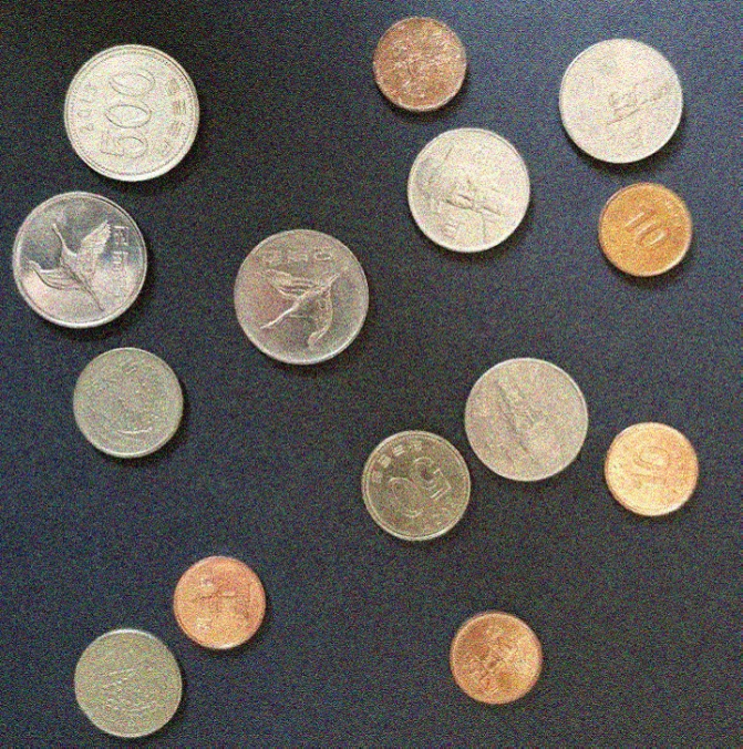
After applying thresholding and morphology, we can identify and extract the target objects from the background by finding the contours around the connected pixels. This technique is used where you need to monitor the number of objects moving on a conveyor belt in an industry process. Goal: Count the number of the individual coins and calculate the total amount of money.

image

Procedure:

1. Apply a filter to remove image noises

2. Choose the appropriate threshold value.

3. Apply the appropriate morphology method to segment coins

4. Find the contour and draw the segmented objects.

5. Exclude the contours which are too small or too big

6. Count the number of each different coins(10/50/100/500 won)

7. Calculate the total amount of money.