Fourier and WaveletTransform
Review of Fourier Analysis
Visualizing Fourier Transform
But what is the Fourier Transform? A visual introduction. - YouTube
Fourier Analysis Lectures
Lecture series by Steve Brunton
Background
Inner Product in Hilbert Space

Side Note
Conjugate:
If a complex number is z=a+bi, where a is the real part and b is the imaginary part, then its conjugate is written as
Normalizing Inner Product
Orthogonal basis functions

Fourier Series

From Fourier Series to Wavelet Functions

Fourier Transformation

Wavelet Decomposition
Wavelet Introduction
Basics of Wavelet
Watch this video for understanding Wavelet transform concept
Wavelets and Multiresolution Analysis - YouTube
Mathematics of Wavelet Transform for Beginners
The Wavelet Transform for Beginners - YouTube
You need to Review Fourier Transform and Short-Time Fourier Transform.
Click here for Review Fourier Transform
Limitation of STFT

Window Function is Finite, so Frequency Resolution decreases.
Fixed length of the window: time and frequency resolution are fixed for entire signals

Narrow Window: Good Time Resolution, Poor Frequency Resolution
Wide Window: Poor Time Resolution, Good Frequency Resolution
Wavelet Transform
Can analyze different Frequency at different Resolution
High frequency signals: apply narrow window
Low frequency signals: apply wide window


Wavelet acts as a scalable and movable window function
Scaling s
Translation tau

Different types of wavelets
Haar, Daubiche, Gaussian, Inverse Mexican Hat etc
Discrete Wavelet Transform
Wavelet transform calculates wavelet coefficients at every possible scale.
This gives a large data
So, use finite numbers of s and \tau
Choose s and \tau based on powers of two for efficient calculation

Multilevel Decomposition

1D Wavelet Decomposition
Algorithms


MATLAB example
wavedec()
**[c,l] = wavedec(x,n,wname) **returns the wavelet decomposition of the 1-D signal x at level n using the wavelet wname.
Dowload Example Code
[c,l] = wavedec(x,n,wname) returns the wavelet decomposition of the 1-D signal x at level n using the wavelet wname. The output decomposition structure consists of the wavelet decomposition vector c and the bookkeeping vector l, which contains the number of coefficients by level. 
Perform a 3-level wavelet decomposition of the signal using the order 2 Daubechies wavelet. Extract the coarse scale approximation coefficients and the detail coefficients from the decomposition.
A = appcoef(C,L,wname) returns the approximation coefficients at the coarsest scale using the wavelet decomposition structure [C,L] of a 1-D signal
D = detcoef(C,L,N) extracts the detail coefficients at the level or levels specified by N.


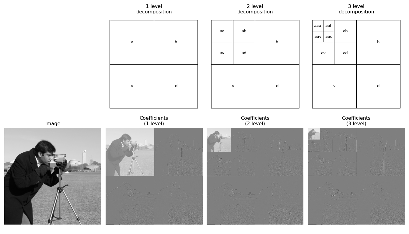
2D Wavelet Decomposition

It can be seen that many of the coefficients are near zero (gray). This ability of the wavelet transform to sparsely represent natural images is a key property that makes it desirable in applications such as image compression and restoration.
For subsequent levels of decomposition, only the approximation coefficients (the lowpass subband) are further decomposed.
The top row indicates the coefficient names as used by
wavedec2()after each level of decomposition. The bottom row shows wavelet coefficients for the camerman image (with each subband independently normalized for easier visualization).
Application
Image Compression using Wavelet
Exercise
Analytical Signal and Hilbert Transform
Analytical Signal and Hilbert Transformation
https://www.gaussianwaves.com/2017/04/analytic-signal-hilbert-transform-and-fft/
Analytical Signal
Continuous Analytical Signal
The analytic signal is complex-valued but its spectrum will be one-sided (only positive frequencies) that preserved the spectral content of the original real-valued signal.

Figure 1: (a) Spectrum of continuous signal x(t) and (b) spectrum of analytic signal z(t)
How to get one-sided Magnitude spectrum?
Frequency domain approach
The one-sided spectrum of $z(t)$ is formed from the two-sided spectrum of the real-valued signal $x(t)$ by applying
Z(f)=⎩⎨⎧X(0)2X(f)0forf=0forf>0forf<0
Time domain approach
Using Hilbert transform approach
One of the important property of an analytic signal is that its real and imaginary components are orthogonal
Discrete Analytical Signal
Discrete-Time Fourier Transform (DTFT).

The analytic signal is complex valued
and should satisfy the following two desired properties
The real part of the analytic signal should be same as the original real-valued signal.
zr[n]=x[n]The real and imaginary part of the analytic signal should satisfy the following property of orthogonality
Given a record of samples x[n] of even length N, the procedure to construct the analytic signal z[n] is as follows.
This method satisfies both the desired properties listed above.
Compute the N-point DTFT of x[n] using FFT
N-point periodic one-sided analytic signal is computed by the following transform
Compute the N-point DTFT of x[n] using FFT ● N-point periodic one-sided analytic signal is computed by the following transform
equation for constructing analytic signal in frequency domain

Finally, the analytic signal (z[n]) is obtained by taking the inverse DTFT of
Envelope (Instantaneous Amplitude) Extraction using Hilbert Transformation
The amplitude modulated signal is
Information bearing signal m(t). Also called instantaneous amplitude.
Carrier signal cos(wc*t)
Similarly, phase or frequency modulations:
The concept of instantaneous phase or instantaneous frequency is required for describing the modulated signal.
General form
Problem statement
Given the modulated signal, extract the instantaneous amplitude (envelope), instantaneous phase and the instantaneous frequency.
The modulated signal is a real-valued signal.
But, amplitude/phase and frequency can be easily computed if the signal is expressed in complex form.
How can we convert a real signal to the complex plane without altering the required properties ?
Apply Hilbert transform and form the analytic signal on the complex plane

The instantaneous amplitude (envelope extraction) is computed in the complex plane as
[

Figure 2: Amplitude modulation using a chirp signal and extraction of envelope and TFS*
MATLAB Tutorial on Envelope Extraction
Last updated