# Tutorial: ODE-IVP
## Part 1: 1st order ODE-IVP problem
Download the MATLAB tutorial source file
* [TU\_ODE\_Part1\_Student\_2024.zip](https://github.com/ykkimhgu/NumericalProg-student/tree/main/tutorial/TU_ODE)
Download the C-prog source file
* [Assigment\_ODE\_student.cpp](https://github.com/ykkimhgu/NumericalProg-student/blob/main/src/Assignment_ODE_student.cpp)
### **Problem**
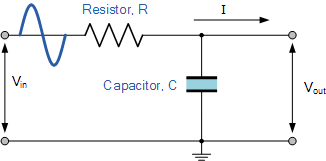
Solve for the response (Vout) of an RC circuit with a sinusoidal input (Vin), from t=0 to 0.1 sec.
where RC=tau=0.01; T=1/tau; f=100; Vm=1; w=2*pi*f;
 ### Tutorial: MATLAB
MATLAB : `ode45()`
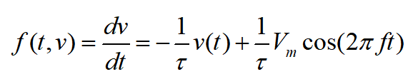
Lets define the RC circuit ODE function f(t,v) as `gradFunc_RC(t,v)`.
```matlab
% Initial Condition
% time
a=0; b=0.1;
h=0.001;
t=a:h:b;
N = (b-a)/h;
% IVP-Initial Condition
v0 = 0;
y0= v0;
%% MATLAB's function ODE45
[tmat,vmat] = ode45(@gradFunc_RC, [a b], v0);
% gradFunc_RC.m
% function dvdt = gradFunc_RC(t,v)
% tau=0.01; f=100; Vm=1;
% dvdt =-v/tau + (1/tau)*Vm*cos(2*pi*f*t);
% end
```
### Analytical Solution (Ground-truth)
The true analytical solution can be expressed as
### Tutorial: MATLAB
MATLAB : `ode45()`
Lets define the RC circuit ODE function f(t,v) as `gradFunc_RC(t,v)`.
```matlab
% Initial Condition
% time
a=0; b=0.1;
h=0.001;
t=a:h:b;
N = (b-a)/h;
% IVP-Initial Condition
v0 = 0;
y0= v0;
%% MATLAB's function ODE45
[tmat,vmat] = ode45(@gradFunc_RC, [a b], v0);
% gradFunc_RC.m
% function dvdt = gradFunc_RC(t,v)
% tau=0.01; f=100; Vm=1;
% dvdt =-v/tau + (1/tau)*Vm*cos(2*pi*f*t);
% end
```
### Analytical Solution (Ground-truth)
The true analytical solution can be expressed as
 ```matlab
% Analytical Solution
tau=0.01; f=100; Vm=1; w=2pif;
A=Vm/(sqrt(1+(wtau)^2));
alpha=-atan(wtau);
v_true=A*(-cos(alpha)exp(-t/tau)+cos(wt+alpha));
```
***
### Exercise
#### **Exercise 1-1: Euler's Explicit Method ( MATLAB)**
```matlab
[t, yE] = odeEU_student(@gradFunc_RC,a,b,h,y0);
figure()
plot(t,yE,'--b',t,v_true,'k')
xlabel('t'); ylabel('v(t)')
```
```matlab
% function [x, yE] = odeEU_student(ODE,a,b,h,y0)
% Variable Initialization
N = (b-a)/h;
yE=zeros(1,N+1);
t=zeros(1,N+1);
% Initial Condition
yE(1) = y0;
t(1)=a;
% Euler Explicit ODE Method
for i = 1:N
% Estimate: yE(i+1)=________
% [TO-DO] your code goes here
% Calculate: t(i+1)=_________
% [TO-DO] your code goes here
end
% end % End of Function
```
#### **Exercise 1-2: Euler's Explicit Method ( C-Prog)**
* Create a project under `\tutorial\Tutorial_ODE\`
* Use the C-prog source template : [Assigment\_ODE\_student.cpp](https://github.com/ykkimhgu/NumericalProg-student/blob/main/src/Assignment_ODE_student.cpp)
* Fill-in the blanks
```c
// Problem1: RC circuit
double odeFunc_rc(const double t, const double v);
// 1st order ODE
void odeEU(double y[], double odeFunc(const double t, const double y),
const double t0, const double tf, const double h, const double y_init);
```
#### Exercise 2: Euler's Modified Method (MATLAB)
```matlab
% Analytical Solution
tau=0.01; f=100; Vm=1; w=2pif;
A=Vm/(sqrt(1+(wtau)^2));
alpha=-atan(wtau);
v_true=A*(-cos(alpha)exp(-t/tau)+cos(wt+alpha));
```
***
### Exercise
#### **Exercise 1-1: Euler's Explicit Method ( MATLAB)**
```matlab
[t, yE] = odeEU_student(@gradFunc_RC,a,b,h,y0);
figure()
plot(t,yE,'--b',t,v_true,'k')
xlabel('t'); ylabel('v(t)')
```
```matlab
% function [x, yE] = odeEU_student(ODE,a,b,h,y0)
% Variable Initialization
N = (b-a)/h;
yE=zeros(1,N+1);
t=zeros(1,N+1);
% Initial Condition
yE(1) = y0;
t(1)=a;
% Euler Explicit ODE Method
for i = 1:N
% Estimate: yE(i+1)=________
% [TO-DO] your code goes here
% Calculate: t(i+1)=_________
% [TO-DO] your code goes here
end
% end % End of Function
```
#### **Exercise 1-2: Euler's Explicit Method ( C-Prog)**
* Create a project under `\tutorial\Tutorial_ODE\`
* Use the C-prog source template : [Assigment\_ODE\_student.cpp](https://github.com/ykkimhgu/NumericalProg-student/blob/main/src/Assignment_ODE_student.cpp)
* Fill-in the blanks
```c
// Problem1: RC circuit
double odeFunc_rc(const double t, const double v);
// 1st order ODE
void odeEU(double y[], double odeFunc(const double t, const double y),
const double t0, const double tf, const double h, const double y_init);
```
#### Exercise 2: Euler's Modified Method (MATLAB)
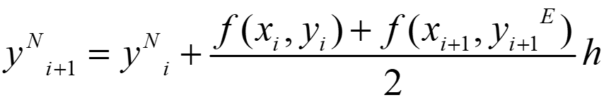 Create `odeEM_student.m`
Modify the given template code
```matlab
[t, yEM] = odeEM_student(@gradFunc_RC,a,b,h,y0);
```
#### Exercise 3-1: 2nd Order Runge-Kutta (MATLAB)
Create `odeEM_student.m`
Modify the given template code
```matlab
[t, yEM] = odeEM_student(@gradFunc_RC,a,b,h,y0);
```
#### Exercise 3-1: 2nd Order Runge-Kutta (MATLAB)
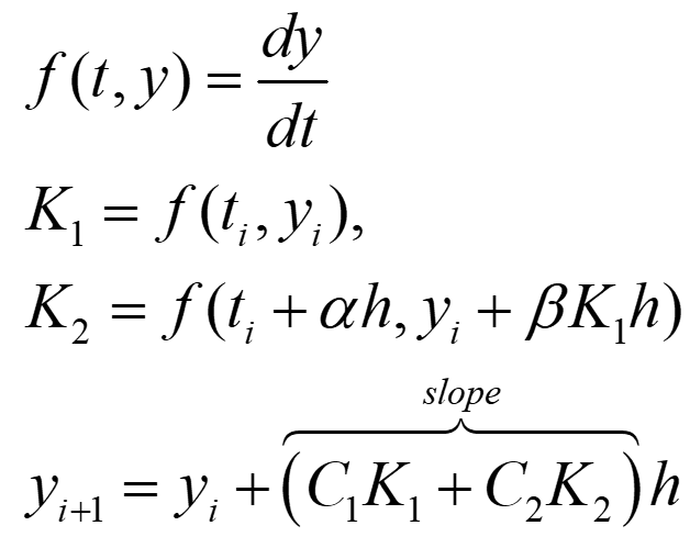 Let alpha=1, C1=0.5, C2=0.5.
Modify the given template code:\\
```matlab
[t, yRK2] = odeRK2_student(@gradFunc_RC,a,b,h,y0);
```
Let alpha=1, C1=0.5, C2=0.5.
Modify the given template code:\\
```matlab
[t, yRK2] = odeRK2_student(@gradFunc_RC,a,b,h,y0);
```
odeRK2_student(odeFunc,a,b,h,y0)
```matlab
function [t, y] = odeRK2_student(odeFunc,a,b,h,y0)
% Variable Initialization
N = (b-a)/h;
y=zeros(1,N+1);
t=zeros(1,N+1);
% Initial Condition
t(1) = a; y(1) = y0;
% RK Design Parameters
alpha=1;
beta=alpha;
C1=0.5;
C2=1-C1;
% ODE Solver
for i = 1:N
t(i+1) = t(i) + h;
% [First-point Gradient]
K1 = odeFunc(t(i),y(i));
% [Second-point Gradient]
% calculate t2=t(i)+alpha*h
% [TO-DO] your code goes here
% t2=___________________
% calculate y2=y(i)+ beta*K1*h
% [TO-DO] your code goes here
% y2=___________________
% Calculate: K2 using t2 and y2
% [TO-DO] your code goes here
% K2=___________________
% Estimate: y(i+1) using RK2
% [TO-DO] your code goes here
% y(i+1)=___________________
end
end % END OF FUNCTION
```
#### Exercise 3-1: 2nd Order Runge-Kutta **( C-Prog)**
* Fill-in the blanks
```c
// 2nd order Runge-Kutta method
void odeRK2(double y[], double odeFunc(const double t, const double y),
const double t0, const double tf, const double h, const double y_init)
```
void odeRK2()
```c
void odeRK2(double y[], double odeFunc(const double t, const double y), const double t0, const double tf, const double h, const double y_init)
{
//
// [BRIEF DESCRIPTION OF THE FUNCTION GOES HERE]
//
// Variable Initialization
int N = (tf - t0) / h + 1;
double y2 = 0;
double t2 = 0;
// Initial Condition
double ti = t0;
y[0] = y_init;
// RK Design Parameters
double C1 = 0.5;
double C2 = 1 - C1;
double alpha = 1;
double beta = alpha;
double K1 = 0, K2 = 0;
// RK2 ODE Solver
for (int i = 0; i < N - 1; i++) {
// [First-point Gradient]
K1 = odeFunc(ti, y[i]);
// [Second-point Gradient]
// Calculate t2=t(i)+alpha*h
// [YOUR CODE GOES HERE]
// t2 =_______________
// Calculate y2 = y(i) + beta * K1 * h
// [YOUR CODE GOES HERE]
// y2 =_______________
// Calculate: K2 using t2 and y2
// [YOUR CODE GOES HERE]
// K2 =_______________
// Estimate: y(i+1) using RK2
// [YOUR CODE GOES HERE]
// y[i + 1] =_______________
ti += h;
}
}
```
##
## Part 2: Higher-order ODE-IVP
Download the tutorial source file
* [TU\_ODE\_Part2\_Student\_2024.zip](https://github.com/ykkimhgu/NumericalProg-student/tree/main/tutorial/TU_ODE)
### **Problem**
Solve for the response of the given system:
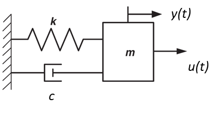
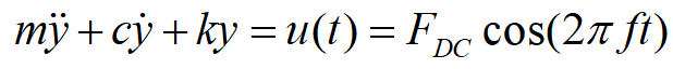 Let, m=1; k=6.9; c=7; f=5;\
u(t)=Fin(t)=2*cos(2*pi*f*t)
### Tutorial: MATLAB
Lets define the mck ODE functions as gradFunc\_mck(t, vecY).
Let, m=1; k=6.9; c=7; f=5;\
u(t)=Fin(t)=2*cos(2*pi*f*t)
### Tutorial: MATLAB
Lets define the mck ODE functions as gradFunc\_mck(t, vecY).
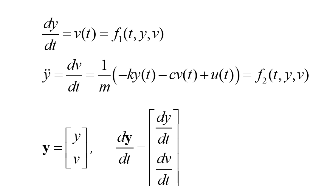 **gradFunc\_mck.m**
```matlab
function [dYdt] = gradFunc_mck(t,vecY)
% Input:
% vecY=[y ; z]
% Output:
% dYdt=[dydt ; dzdt]
% Variable Initialization
dYdt=zeros(2,1);
% System Modeling parameters
m=1; k=6.9; c=10*0.7;
FinDC=2; f=5;
Fin=FinDC*cos(2*pi*f*t);
% Output
dYdt(1)=vecY(2);
dYdt(2)=1/m*(Fin-c*vecY(2)-k*vecY(1));
end
```
**MATLAB : ode45()**
```matlab
% Initial Condition
% time
a=0;
b=1;
h=0.01;
N = (b-a)/h;
% IVP-Initial Condition
yINI = 0;
vINI = 0.2;
% ODE Solver
[tref, vecY] = ode45(@gradFunc_mck, [a:h:b], [yINI, vINI]);
```
### Exercise
#### Exercise 1: Euler's Explicit Method for 2nd-order ODE (MATLAB)
**sys2EU\_student.m**
First, fill-in this blank and complete the algorithm
**gradFunc\_mck.m**
```matlab
function [dYdt] = gradFunc_mck(t,vecY)
% Input:
% vecY=[y ; z]
% Output:
% dYdt=[dydt ; dzdt]
% Variable Initialization
dYdt=zeros(2,1);
% System Modeling parameters
m=1; k=6.9; c=10*0.7;
FinDC=2; f=5;
Fin=FinDC*cos(2*pi*f*t);
% Output
dYdt(1)=vecY(2);
dYdt(2)=1/m*(Fin-c*vecY(2)-k*vecY(1));
end
```
**MATLAB : ode45()**
```matlab
% Initial Condition
% time
a=0;
b=1;
h=0.01;
N = (b-a)/h;
% IVP-Initial Condition
yINI = 0;
vINI = 0.2;
% ODE Solver
[tref, vecY] = ode45(@gradFunc_mck, [a:h:b], [yINI, vINI]);
```
### Exercise
#### Exercise 1: Euler's Explicit Method for 2nd-order ODE (MATLAB)
**sys2EU\_student.m**
First, fill-in this blank and complete the algorithm
function [t, yE, vE] = sys2EU_student()
```matlab
% function [t, yE, vE] = sys2EU_student(gradF,a,b,h,yINI, vINI)
% Variable Initialization
N = (b-a)/h;
t=zeros(1,N+1);
yE=zeros(1,N+1);
vE=zeros(1,N+1);
% Initial Condition
yE(1) = yINI;
vE(1) = vINI;
t(1)=a;
% Euler Explicit ODE Method
for i = 1:N
t(i+1) = t(i) + h;
dYdt=gradFunc_mck(t(i),[yE(i),vE(i)]);
% Estimate: yE(i+1)=________
% [TO-DO] your code goes here
% Estimate: vE(i+1)=________
% [TO-DO] your code goes here
end
% end % End of Function
```
Then, create the function file as `sys2EU_student.m`
`[t, yE, vE] = sys2EU_student(@gradFunc_mck,a,b,h,yINI, vINI);`
#### Exercise 2-1: 2nd order Runge-Kutta for 2nd-order ODE (MATLAB)
Create `sys2RK2_student.m`
Modify the given template code
```matlab
[t, yRK2, vRK2] = sys2RK2_student(@mckFunc,a,b,h,yINI,vINI);
```
#### Exercise 2-2: 2nd order Runge-Kutta for 2nd-order ODE (C-Prog)
Fill-in this blank and complete the algorithm
```cpp
void sys2RK2(double y1[], double y2[],
void odeFuncSys(double dYdt[], const double t, const double Y[]),
const double t0, const double tf, const double h, const double y1_init,
const double y2_init);
```
***
## Assignment
### Q1. Create C/C++ function for 1st order ODE
#### Use 2nd, 3rd order Runge-Kutta method
```c
// 2nd order Runge-Kutta method
void odeRK2(double y[], double odeFunc(const double t, const double y),
const double t0, const double tf, const double h, const double y_init)
// 3rd order Runge-Kutta method
void odeRK3 (double y[], double odeFunc(const double t, const double y),
const double t0, const double tf, const double h, const double y_init)
```
> For RK2, use alpha=1, C1=0.5
>
> For RK3, use classical third-order Runge-Kutta
### Q2. Create C/C++ function for 2nd order ODE
#### Use 2nd order Runge-Kutta method
```cpp
void sys2RK2(double y1[], double y2[],
void odeFuncSys(double dYdt[], const double t, const double Y[]),
const double t0, const double tf, const double h, const double y1_init,
const double y2_init);
```